(This post was originally published in Generalized Method of Moments (GMM) in R (Part 2 of 3). I rewrite it here to utilize markdown and latex for scientific post.)
This is the second post of the series about GMM, short for Generalized Method of Moments in Econometrics and Statistics. Interested audience are welcomed to review my last post Generalized Method of Moments (GMM) in R (Part 1 of 3) for the basic ideas of GMM and the application using R package gmm. In the last post, it is illustrated that OLS estimator is just GMM estimator, so exactly the same point estimates of OLS as those of GMM can be observed for the same set of data under the case of linear regression. However, the computed standard errors for OLS are usually different from those returned by gmm package, because by default gmm at least allows for heteroskedasticity across samples but the standard errors for the usual OLS function usually depend on homoskedasticity. That is, gmm just provides the same point estimates as those of OLS but more robust standard errors than those of OLS. Admittedly, the discussion of OLS needs not explicitly touch GMM in the first course of Econometrics. Even for application, it is still fine to demonstrate the robust standard errors for OLS estimators directly without bothering GMM. However, as I said before GMM just provides another view to construct the omnibus system for the extremum estimator and another angle to view what we have learned for OLS and MLE. In terms of the application about structural models, GMM is a natural method for estimation which only requires the validity of moment conditions. Generally speaking, such moment conditions can be derived by the related theories of domain knowledge (e.g. Economics, Marketing, etc.) In next post, I will try illustrating GMM for endogeneity problem for structural models. However, in this post I still hope to start with what we are familiar with to comprehend GMM.
In this post why MLE estimator is also GMM estimator is discussed. On the other hand several experiments are also conducted to illustrate the weird behaviors of optim() in R, and then it is highly recommended to avoid using it.
MLE as GMM
Just mimic the ideas in the discussion about OLS as GMM in the last post, and here why MLE estimator is just GMM estimator is illustrated. The central point for this statement is about the construction of moment conditions for general application of MLE.
One may recall that in the discussion about OLS as GMM I just go to the linear projection model which inspires OLS, instead of OLS directly. Actually this is one of the illustration styles about extremum estimators in Hansen’s textbooks (Econometrics and Probability and Statistics for Economists). That is, we can build up a general way to construct estimators as sample analogs of population parameters. Therefore, linear projection model is illustrated for the sensible Linear Projection Coefficient \(\boldsymbol{\beta}\) to minimize mean squared prediction error (MSE): \(S(\boldsymbol{\beta})=\mathbb{E}\left[\left(y-\boldsymbol{x}^{\prime} \boldsymbol{\beta}\right)^{2}\right]\). Based on such conceptual population model, the sample analog of MSE is just the sum-of-squared-errors:
\[\begin{gathered} \widehat{S}(\boldsymbol{\beta})=\frac{1}{n} \sum_{i=1}^{n}\left(y_{i}-\boldsymbol{x}_{i}^{\prime} \boldsymbol{\beta}\right)^{2} \\ =\frac{1}{n} \operatorname{SSE}(\boldsymbol{\beta}) \\ \text { where } \operatorname{SSE}(\boldsymbol{\beta})=\sum_{i=1}^{n}\left(y_{i}-\boldsymbol{x}_{i}^{\prime} \boldsymbol{\beta}\right)^{2} \end{gathered}\]Therefore, OLS estimator is just the sample analog of Linear Projection Coefficient \(\boldsymbol{\beta}\), since Linear Projection Coefficient \(\boldsymbol{\beta}\) minimizes mean squared prediction error (MSE): \(S(\boldsymbol{\beta})=\mathbb{E}\left[\left(y-\boldsymbol{x}^{\prime} \boldsymbol{\beta}\right)^{2}\right]\) and OLS estimator minimizes sum-of-squared-errors. One of the benefits for doing so is to facilitate the construction about population moment conditions for GMM and then indicate the relation between OLS estimator and GMM estimator. The basic reason is that they both can be traced to the common population moment conditions:
\[\mathbb{E}[\boldsymbol{x} e] = \boldsymbol{0}\]It is also useful to show that the MLE is a sample analog of the true parameter in terms of the log likelihood function for the population model. It is useful to starts with the joint likelihood:
\[f(y, \boldsymbol{x} ; \boldsymbol{\theta})=f(y \mid \boldsymbol{x} ; \boldsymbol{\theta}) \times f(\boldsymbol{x})\]In general, the regular assumption is made so that the conditional likelihood is the only focus, and it is also useful to define the expected log density function:
\[l(\boldsymbol{\theta})=\mathbb{E}[\log f(y \mid \boldsymbol{x} ; \boldsymbol{\theta})]\]to remove the randomness from \(y\) and \(\boldsymbol{x}\) such that it is the function of the parameter \(\boldsymbol{\theta}\). One important theorem is that when the model is correctly specified the true parameter \(\boldsymbol{\theta}_0\) maximizes the expected log density \(l(\boldsymbol{\theta})\). One can check the technical issues about this theorem in Section 10.20 of Probability and Statistics for Economists (Hansen, Bruce E., 2021). The basic idea is straightforward. If the assumptions about the data generation process and the distributions are reliable, then the true parameters should be consistent with such assumptions to maximize \(l(\boldsymbol{\theta})\) This idea just inspires MLE just as the idea of linear projection model inspires OLS. That is, MLE estimator is analog to \(\boldsymbol{\theta}_{0}\) since MLE estimator maximizes the sample analog of \(l(\boldsymbol{\theta})\):
\[\bar{\ell}_{n}(\theta)=\frac{1}{n} \ell_{n}(\theta)=\frac{1}{n} \sum_{i=1}^{n} \log f\left(X_{i} \mid \theta\right)\]In terms of the optimization problem for the expected log density function, the first order condition is
\[\mathbb{E}\left[\frac{d}{d \theta} \log f(y \mid \boldsymbol{x} ; \boldsymbol{\theta})\right]=\mathbf{0}\]which are just the population moment conditions for GMM. Similarly, the corresponding sample moment conditions are also just the direct results of first order condition of the maximization of the sample log likelihood
\[\frac{1}{n} \sum_{i=1}^{n} \frac{d}{d \theta} \log f\left(y_{i} \mid x_{i} ; \theta\right)=\mathbf{0}\]Therefore, MLE estimator is just GMM estimator, and actually it is the MM estimator since the number of moment conditions is that same as the number of unknowns.
The next question is whether the covariance of MLE estimator is the same as that of GMM estimator. The short answer is, no. The basic reason is that under MLE the distributional assumptions are made for the data generation process but GMM does ONLY require moment conditions. Therefore, GMM covariance is again more robust than MLE covariance. Here is the illustration with some mathematics. With the general discussion about the GMM in the last post, GMM estimator has the following sampling distribution:
\(\sqrt{N}(\hat{\theta}-\theta) \rightarrow \mathcal{N}(0, V)\) where \(V=I(\theta)^{-1} J(\theta) I(\theta)^{-1}\) with \(I(\theta) \equiv \lim _{N \rightarrow \infty} \frac{1}{N} \sum_{i=1}^{N} I_{i}(\theta) \quad \text { and } \quad J(\theta) \equiv \lim _{N \rightarrow \infty} \frac{1}{N} \sum_{i=1}^{N} J_{i}(\theta)\) where \(I_{i}(\theta)=E\left\{-\frac{\partial s_{i}(\theta)}{\partial \theta^{\prime}}\right\}=E\left\{-\frac{\partial^{2} \log L_{i}(\theta)}{\partial \theta \partial \theta^{\prime}}\right\}\)
As discussed in the last post \(J(\theta)\) is actually the optimal weight matrix, which is the covariance of moment conditions:
\[J_{i}(\theta)=E\left\{s_{i}(\theta) s_{i}(\theta)\right\}\]From the textbook discussion about MLE, we know that the \(I(\theta)\) is called information matrix, which is the hessian of the log likelihood. Furthermore, if the distributional assumption is valid, then we have information equality: \(I(\theta)=J(\theta)\). That is, MLE estimator just explicitly depends on the distributional assumption, so the covariance is \(I^{-1}\). Therefore, GMM covariance is generally more robust than MLE covariance, since it does not expect the information equality relying on the validity of distributional assumption.
Case Study Again for R&D Data
Just return to the data about R&D from Section 7.3.2 of A Guide to Modern Econometrics (2nd edition), and try conducting MLE and GMM on it. In general, one can easily conceive that the number of patents are discrete and only non negative, so the specific distribution can be made, e.g. Poisson. Actually the Poisson model just describes the conditional distribution of the number of patents as
\[P\left\{y_{i}=y \mid x_{i}\right\}=\frac{\exp \left\{-\lambda_{i}\right\} \lambda_{i}^{y}}{y !}, \quad y=0,1,2, \ldots\]where
\[\lambda_{i} \equiv \exp \left\{x_{i}^{\prime} \beta\right\}\]is also the conditional mean of such Poisson distribution. Since it is no longer the simple linear model and specific distributional assumption is made, MLE is the natural choice to estimate the parameters. It is quite easy to get the results in R:
poisson_res <- patents_df %>%
  glm(p91 ~ lr91 + aerosp + chemist + computer + machines +
    vehicles + japan + us, family = poisson(), data = .)
summary(poisson_res)
and the results are
Call:
glm(formula = p91 ~ lr91 + aerosp + chemist + computer + machines +
    vehicles + japan + us, family = poisson(), data = .)

Deviance Residuals:
    Min       1Q   Median       3Q      Max
-27.979   -5.246   -1.572    2.352   29.246

Coefficients:
             Estimate Std. Error z value Pr(>|z|)
(Intercept) -0.873731   0.065868  -13.27  < 2e-16 ***
lr91         0.854525   0.008387  101.89  < 2e-16 ***
aerosp      -1.421850   0.095640  -14.87  < 2e-16 ***
chemist      0.636267   0.025527   24.93  < 2e-16 ***
computer     0.595343   0.023338   25.51  < 2e-16 ***
machines     0.688953   0.038346   17.97  < 2e-16 ***
vehicles    -1.529653   0.041864  -36.54  < 2e-16 ***
japan        0.222222   0.027502    8.08 6.46e-16 ***
us          -0.299507   0.025300  -11.84  < 2e-16 ***
---
Signif. codes:  0 ‘***’ 0.001 ‘**’ 0.01 ‘*’ 0.05 ‘.’ 0.1 ‘ ’ 1

(Dispersion parameter for poisson family taken to be 1)

    Null deviance: 29669.4  on 180  degrees of freedom
Residual deviance:  9081.9  on 172  degrees of freedom
AIC: 9919.6

Number of Fisher Scoring iterations: 5
However, Poisson distribution is often too strong and its direct property is equidispersion, which describes the equality of mean and variance for each sample. If this is the case, the first question is whether the MLE estimator is still reliable, or say, consistent? From the above discussion, MLE estimator is just GMM estimator and the consistency of GMM estimator only depends on the validity of moment conditions. So, let’s check the corresponding moment conditions. In terms of this case, one can just argue that the conditional expectation is assumed to have the \(\exp()\) form:
\[E\left\{y_{i} \mid x_{i}\right\}=\exp \left\{x_{i}^{\prime} \beta\right\}\]Therefore, we can have the following constructed error
\[\varepsilon_{i}=y_{i}-\exp \left\{x_{i}^{\prime} \beta\right\}\]satisfying
\[E\left\{\varepsilon_{i} \mid x_{i}\right\}=0\]Therefore, \(E\left\{\varepsilon_{i} x_{i}\right\}=0\)
Accordingly, the sample moment conditions are
\[\sum_{i=1}^{N}\left(y_{i}-\exp \left\{x_{i}^{\prime} \beta\right\}\right) x_{i}=\sum_{i=1}^{N} \varepsilon_{i} x_{i}=0\]which is also the first order condition for the log likelihood maximization with the Poisson distribution assumed. That is, it is also the sample moment conditions for the corresponding GMM estimator for such Poisson MLE model. Therefore, if we can trust the specified functional form of conditional expectation, then the consistency of GMM estimator is reliable and thus the consistency of MLE estimator is too. This is the magical part of the conclusion: even if the conditional distribution of y does not follow Poisson distribution, Poisson MLE estimator is still consistent based on the condition that the conditional expectation is assumed to have the \(\exp()\) form:
\[E\left\{y_{i} \mid x_{i}\right\}=\exp \left\{x_{i}^{\prime} \beta\right\}\]In literature, we refer to the estimator as a quasi-maximum likelihood estimator (QMLE). Quasi usually means not real. Apparently such estimator is derived from the Poisson distribution, but actually it can also be derived by the moment conditions relying on the specification of conditional expectation.
In terms of the estimates of covariance matrix, one can perceive that MLE procedure only returns \(I^{-1}\) but GMM procedure should return
\[V=I(\theta)^{-1} J(\theta) I(\theta)^{-1}\]which is more robust. With gmm, one can easily construct the moment conditions:
# GMM estimator as Quasi- (Psudo-) MLE
# Define moment conditions matrix for QMLE (gmm)
mom <- function(beta, df) {
  # df is the data frame with first column as dv
  # This function returns n * q matrix
  # Each column is one moment condition before taking sample average
  # There are totally q moment conditions
y <- as.numeric(df[, 1])
  x <- data.matrix(df[, 2:ncol(df)])
# Refer to moment conditions of QMLE
  m <- x * as.vector(y - exp(x %*% beta))
return(cbind(m))
}
# Generate regression coef as the initial values for QMLE (gmm)
init_values <- patents_df %>%
  select(
    p91, lr91, aerosp, chemist, computer, machines,
    vehicles, japan, us
  ) %>%
  mutate(const = 1) %>%
  # Please hold the order as previous glm() to facilitate comparison
  select(
    p91, const, lr91, aerosp, chemist, computer, machines,
    vehicles, japan, us
  ) %>%
  lm(p91 ~ lr91 + aerosp + chemist + computer + machines +
    vehicles + japan + us, data = .) |>
  {\(x) coef(x)*0.01}()
# Be careful that we need to use "nlminb" INSTEAD OF "optim", which is
# bloody awful.
# Refer to https://cran.r-project.org/web/packages/gmm/vignettes/gmm_with_R.pdf
# Just use random initial values
set.seed(1024)
qmle_res_1 <- gmm(mom, df_n, rnorm(length(init_values)),
  wmatrix = "optimal",
  vcov = "MDS",
  optfct = "nlminb",
  control = list(eval.max = 10000)
)
summary(qmle_res_1)
and the results are
Call:
gmm(g = mom, x = df_n, t0 = rnorm(length(init_values)), wmatrix = "optimal",
    vcov = "MDS", optfct = "nlminb", control = list(eval.max = 10000))


Method:  twoStep

Kernel:  Quadratic Spectral

Coefficients:
          Estimate     Std. Error   t value      Pr(>|t|)
Theta[1]  -8.7373e-01   7.4295e-01  -1.1760e+00   2.3958e-01
Theta[2]   8.5453e-01   9.3694e-02   9.1204e+00   7.4878e-20
Theta[3]  -1.4219e+00   3.8016e-01  -3.7401e+00   1.8395e-04
Theta[4]   6.3627e-01   2.2536e-01   2.8234e+00   4.7520e-03
Theta[5]   5.9534e-01   3.0080e-01   1.9792e+00   4.7795e-02
Theta[6]   6.8895e-01   4.1468e-01   1.6614e+00   9.6628e-02
Theta[7]  -1.5297e+00   2.8069e-01  -5.4496e+00   5.0489e-08
Theta[8]   2.2222e-01   3.5284e-01   6.2981e-01   5.2882e-01
Theta[9]  -2.9951e-01   2.7362e-01  -1.0946e+00   2.7368e-01

J-Test: degrees of freedom is 0
                J-test                P-value
Test E(g)=0:    4.82602870693394e-15  *******

#############
Information related to the numerical optimization
Convergence code =  0
Function eval. =  83
Gradian eval. =  515
Message:  X-convergence (3)
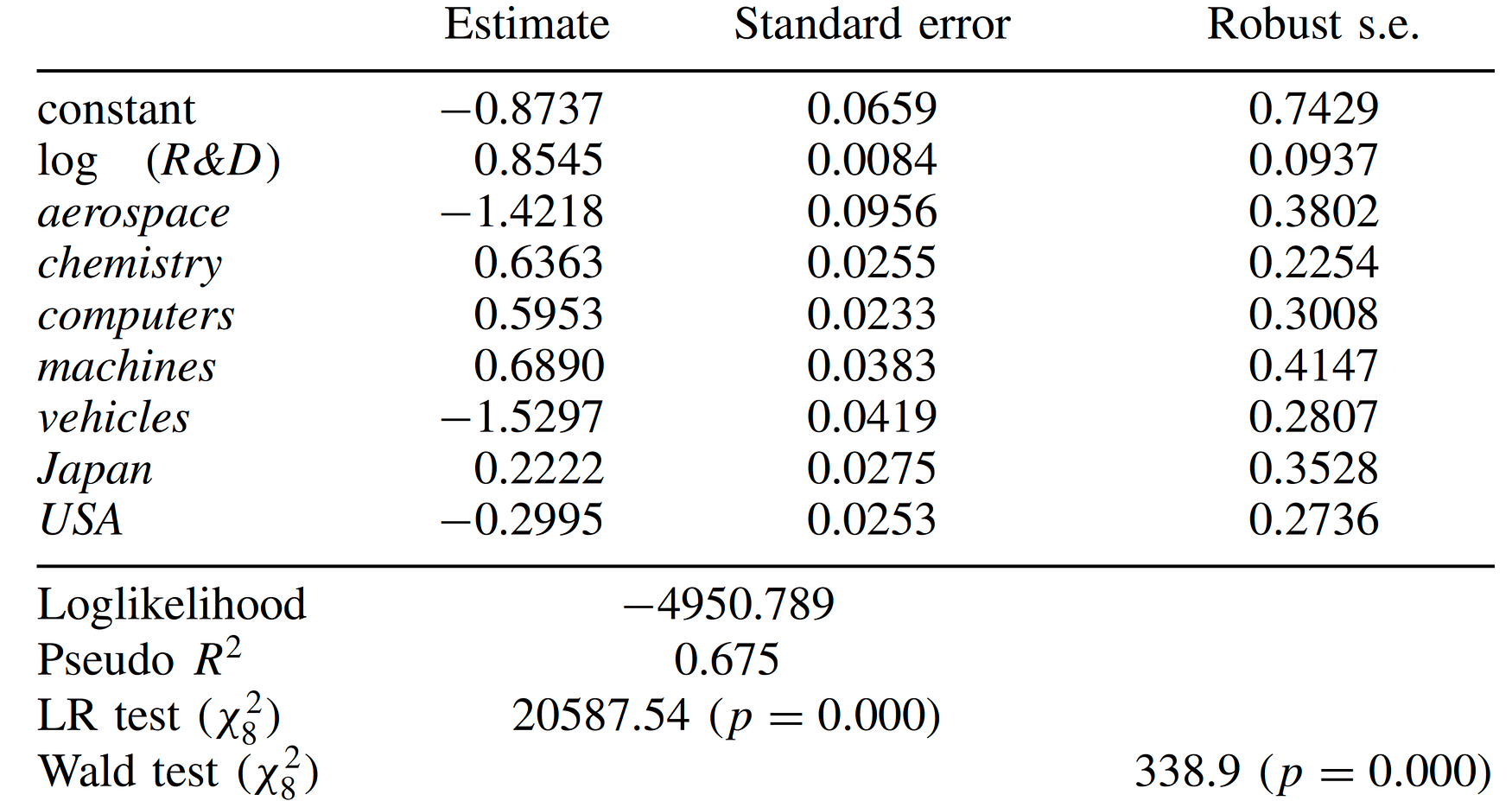
One can find that the points estimates are the same as those from MLE but the covariances differ. One can check that we just replicate the results in the table in P216 of A Guide to Modern Econometrics:
Instability of optim() in R
Until now, it is always emphasized to select "nlminb" for optfnc instead of the default optim. One can check the experiments when using optim for the problem and the incorrect results are found:
# Just use random initial values
set.seed(1024)
qmle_res_3 <- gmm(mom, df_n, rnorm(length(init_values)),
  wmatrix = "optimal",
  vcov = "MDS",
  optfct = "optim",
  control = list(maxit = 10000)
)
summary(qmle_res_3)
and the results are
Call:
gmm(g = mom, x = df_n, t0 = rnorm(length(init_values)), wmatrix = "optimal",
    vcov = "MDS", optfct = "optim", control = list(maxit = 10000))


Method:  twoStep

Kernel:  Quadratic Spectral

Coefficients:
          Estimate     Std. Error   t value      Pr(>|t|)
Theta[1]   4.68677922   1.27672054   3.67095152   0.00024165
Theta[2]   0.11570739   0.19122828   0.60507468   0.54512938
Theta[3]  -3.27941695   2.04110024  -1.60669079   0.10812222
Theta[4]  -0.22722767   0.33122546  -0.68602113   0.49269979
Theta[5]   0.34977317   0.32271631   1.08384100   0.27843530
Theta[6]  -1.29893740   1.31655110  -0.98662133   0.32382831
Theta[7]  -4.52432887   4.93624197  -0.91655330   0.35937677
Theta[8]   0.66823830   0.42017527   1.59037989   0.11174920
Theta[9]  -1.19538287   0.43457120  -2.75071811   0.00594648

J-Test: degrees of freedom is 0
                J-test            P-value
Test E(g)=0:    24521.7280884245  *******

#############
Information related to the numerical optimization
Convergence code =  0
Function eval. =  1558
Gradian eval. =  NA
and
# What about anoter set of random initial values
set.seed(4201)
qmle_res_4 <- gmm(mom, df_n, rnorm(length(init_values)),
  wmatrix = "optimal",
  vcov = "MDS",
  optfct = "optim",
  control = list(maxit = 10000)
)
summary(qmle_res_4)
and the results are
Call:
gmm(g = mom, x = df_n, t0 = rnorm(length(init_values)), wmatrix = "optimal",
    vcov = "MDS", optfct = "optim", control = list(maxit = 10000))


Method:  twoStep

Kernel:  Quadratic Spectral

Coefficients:
          Estimate     Std. Error   t value      Pr(>|t|)
Theta[1]  -2.2705e+00   8.8977e-01  -2.5518e+00   1.0717e-02
Theta[2]   1.0505e+00   1.0605e-01   9.9060e+00   3.9217e-23
Theta[3]   1.2665e+00   4.5386e-01   2.7904e+00   5.2639e-03
Theta[4]   8.2098e-01   2.7199e-01   3.0184e+00   2.5414e-03
Theta[5]   1.0493e+00   3.2657e-01   3.2130e+00   1.3134e-03
Theta[6]   1.0738e+00   5.0875e-01   2.1106e+00   3.4806e-02
Theta[7]  -1.7693e+00   3.8303e-01  -4.6194e+00   3.8490e-06
Theta[8]  -1.1773e-01   3.7078e-01  -3.1752e-01   7.5085e-01
Theta[9]  -6.2103e-01   3.0085e-01  -2.0643e+00   3.8991e-02

J-Test: degrees of freedom is 0
                J-test            P-value
Test E(g)=0:    7532.64472252297  *******

#############
Information related to the numerical optimization
Convergence code =  0
Function eval. =  846
Gradian eval. =  NA
One can find that the optimization outcome just indicates that it successfully converges, but the results are incorrect! This is just the MM estimator, so the value should be 0! To be honest, such findings just astonished me when I prepared for the lecture notes. So far as I know, many R packages still use optim() for numerical optimization, but from these experiences it is suggested to be careful and not to use it whenever possible.
Summary
In this post, the relation between MLE and GMM is discussed. Actually MLE estimator is also GMM estimator, and the consistency of MLE estimator can still hold if the consistency of GMM estimator can hold. In the R&D example shown in the post, one can still argue for the consistency when Poisson distribution is challenged if the \(\exp()\) specification of the condition expectation is acceptable. On the other hand, GMM procedure can provides more robust covariance when the data generation process does not follow Poisson distribution.
On the other hand, from the experiments I also find the instability of optim() which is the usual R function for numerical optimization. The disaster is that so far as I know many packages on Econometrics or statistics usually employ optim(), so one should be careful for the future usage of such packages. The lucky point is that currently we have alternatives. In the post for gmm I just switch to nlminb. I believe other R packages should have similar options for the optimization methods. For those who would like to conduct the studies about computational topics, Julia is recommended for trials. Well, I just bothered Rcpp some years ago to have two-language problems. Julia is expected to deal with such problems to balance easy coding and fast speed.
References
-
Chaussé, P. (2021). Computing generalized method of moments and generalized empirical likelihood with R. Journal of Statistical Software, 34(11), 1–35.
-
Chausse, P., & Chausse, M. P. (2021). Package ‘gmm’.
-
Verbeek, M. (2004). A Guide to Modern Econometrics (2nd edition). ERIM (Electronic) Books and Chapters. John Wiley&Sons, Chichester.
-
Hansen, Bruce E. (2021). Econometrics. Typescript, University of Wisconsin. Princeton University Press, forthcoming.
-
Hansen, Bruce E. (2021). Probability and Statistics for Economists. Typescript, University of Wisconsin. Princeton University Press, forthcoming.
-
White, H. (1980). A heteroskedasticity-consistent covariance matrix estimator and a direct test for heteroskedasticity. Econometrica: journal of the Econometric Society, 817-838.